HMM
The HMM method can be used to determine the essentiality of the entire genome, as opposed to gene-level analysis of the other methods. It is capable of identifying regions that have unusually high or unusually low read counts (i.e. growth advantage or growth defect regions), in addition to the more common categories of essential and non-essential.
Note
Intended only for Himar1 datasets.
How does it work?
Usage
> python3 transit.py hmm <comma-separated .wig files> <annotation .prot_table or GFF3> <output_BASE_filename>
      (will create 2 output files: BASE.sites.txt and BASE.genes.txt)

      Optional Arguments:
          -r <string>     :=  How to handle replicates. Sum, Mean. Default: -r Mean
          -l              :=  Perform LOESS Correction; Helps remove possible genomic position bias. Default: Off.
          -iN <float>     :=  Ignore TAs occuring at given percentage (as integer) of the N terminus. Default: -iN 0
          -iC <float>     :=  Ignore TAs occuring at given percentage (as integer) of the C terminus. Default: -iC 0
Parameters
The HMM method automatically estimates the necessary statistical parameters from the datasets. You can change how the method handles replicate datasets:
Replicates: Determines how the HMM deals with replicate datasets by either averaging the read-counts or summing read counts across datasets. For regular datasets (i.e. mean-read count > 100) the recommended setting is to average read-counts together. For sparse datasets, it summing read-counts may produce more accurate results.
Output and Diagnostics
Column # |
Column Definition |
|---|---|
1 |
Coordinate of TA site |
2 |
Observed Read Counts |
3 |
Probability for ES state |
4 |
Probability for GD state |
5 |
Probability for NE state |
6 |
Probability for GA state |
7 |
State Classification (ES = Essential, GD = Growth Defect, NE = Non-Essential, GA = Growth-Defect) |
8 |
Gene(s) that share(s) the TA site. |
Column Header |
Column Definition |
|---|---|
Orf |
Gene ID |
Name |
Gene Name |
Desc |
Gene Description |
N |
Number of TA sites |
n0 |
Number of sites labeled ES (Essential) |
n1 |
Number of sites labeled GD (Growth-Defect) |
n2 |
Number of sites labeled NE (Non-Essential) |
n3 |
Number of sites labeled GA (Growth-Advantage) |
Avg. Insertions |
Mean insertion rate within the gene |
Avg. Reads |
Mean read count within the gene |
State Call |
State Classification (ES = Essential, GD = Growth Defect, NE = Non-Essential, GA = Growth-Defect) |
Run-time
HMM Confidence Scores (Oct 2023)
One of the difficulties in assessing the certainties of the HMM calls is that, while the formal state probabilities are calculated at individual TA sites, the essentiality calls at the gene level are made by taking a vote (the most frequent state among its TA sites), and this does not lend itself to such formal certainty quantification. However, we developed a novel approach to evaluating the confidence of the HMM calls for genes. We have sometimes noticed that short genes are susceptible to being influenced by the essentiality of an adjacent region, which is evident by examining the insertion statistics (saturation in gene, or percent of TA sites with insertion, and mean insertion count at those sites). For example, consider a hypothetical gene with just 2 TA sites that is labeled as ES by the HMM but has insertions at both sites. It might be explained by proximity to a large essential gene or region, due to the “smoothing” the HMM does across the sequence of TA sites. Thus we can sometimes recognize inaccurate calls by the HMM if the insertion statistics of a gene are not consistent with the call (i.e. a gene labeled as NE that has no insertions, or conversely, a gene labeled ES that has many insertion).
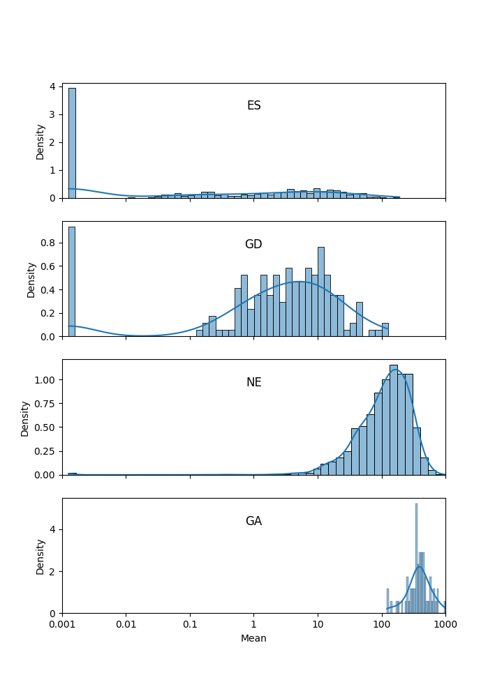
In our paper on the HMM in Transit (DeJesus et al, 2013), we showed a plot of random samples from the joint posterior distribution of local saturation and mean insertion counts (at non-zero sites) for the 4 essentiality states, which nicely demonstrates that that ES genes have near-0 saturation and low counts at non-zero sites, NE genes have high saturation and counts, GD genes fall in between, and GA genes are almost fully saturated with excessively high counts.
Following this idea, we can use the observed insertion counts in each gene to assess the confidence in each of the essentiality calls by the HMM. Rather than modeling them as 2D distributions, we combine them into 1D (Gaussian) distributions over the overall mean insertion count in each gene, including sites with zeros. The mean count for essential (ES) genes usually around 0, typically around 5-10 for growth-defect (GD) genes, around 100 for non-essential (NE) genes, and >300 for growth-advantaged (GA) genes (assuming TTR normalization, by default).
We now calculate these conditional distributions empirically for each dataset on which the HMM is run, and use it to assess the confidence in each of the essentiality calls. We start by calculating the mean and standard deviation of saturation and insertion count over all the genes in each of the 4 states (ES, GD, NE, and GA). The empirical mean and standard deviation for each state are reported in the header of the output file (by HMM_conf.py, see below). Then, for each gene, we compute the probability density (likelihood) of its mean count with respect to the Normal distribution for each of the 4 states. For example, suppose a gene g is called state s. Then:
P(g|s) = N(cnt(g)|μ_cnt(s), σ_cnt(s))
The 4 probabilities are normalized to sum up to 1. The confidence in the HMM call for a gene is taken to be the normalized probability of the called state.
This confidence score nicely identifies genes of low confidence, where the local saturation and mean insertion count seem inconsistent with the HMM call. The low-confidence genes are biased toward short genes (with 1-3 TA sites), though they include some large genes with many TA sites as well. Some of the former are cases where the call of a short gene is influenced by an adjacent region. Some of the latter include ambiguous cases like multi-domain proteins, where one domain is essential and the other is not. We observed that there are often “borderline” (or ambiguous) genes, where the called state has significant probability (>0.2), but is not the most probable state (i.e. another state is more likely, based on the insertions in the gene).
- Criteria (for gene g with called state c):
genes where the called state has the highest conditional probability (most likely, given their mean count) are ‘confident’
genes where P(g|c)>0.2, but there is another state that has higher probability are ‘ambiguous’
genes with P(g|c)<0.2 are ‘low-confidence’
The ‘low-confidence’ and ‘ambiguous’ genes are now indicated in the ‘flag’ field added by HMM_conf.py in the output files (see below).
In genomes with thousands genes, it is not uncommon for there to be a few hundred low-confidence and ambiguous genes each, depending on the saturation of the input dataset (.wig file); less-saturated datasets tend to have more low-confidence genes.
We implemented this procedure as a stand-alone post-processing script (called ‘HMM_conf.py’ in the src/ directory) which is run on HMM output files, calculates a “confidence” score for each gene and appends this information as extra columns to the HMM output file. (In the future, it will be integrated directly into the HMM output, obviating the need for a second step.)
usage: python3 src/HMM_conf.py <HMM_output.genes.txt>

example:

> python HMM_conf.py HMM_Ref_sync3_genes.txt > HMM_Ref_sync3_genes.conf.txt
The script adds the following columns:
consis - consistency (proportion of TA sites representing the majority essentiality state)
If consistency<1.0, it means not all the TA sites in the gene agree with the essentiality call, which is made by majority vote. It is OK if a small fraction of TA sites in a gene are labeled otherwise. If it is a large fraction (consistency close to 50%), it might be a ‘domain-essential’ (multi-domain gene where one domain is ES and the other is NE).
probES - conditional probability (normalized) of the mean insertion count if the gene were essential
probGD - conditional probability (normalized) of the mean insertion count if the gene were growth-defect (i.e. disruption of gene causes a growth defect)
probNE - conditional probability (normalized) of the mean insertion count if the gene were non-essential
probGA - conditional probability (normalized) of the mean insertion count if the gene were growth-advantaged
conf - confidence score (normalized conditional joint probability of the insertion statistics, given the actual essential call made by the HMM)
flag - genes that are ambiguous or have low confidence are labeled as such:
low-confidence means the proability of the HMM call is <0.2 based on the mean insertion counts in gene, so the HMM call should be ignored
ambiguous means the called state has prob>0.2, but there is another state with higher probability; these could be borderline cases where the gene could be in either category
Here is an example to show what the additional columns look like. The Mean insertion counts for the 4 essentiality states can be seen in the header. Note that MAB_0005 was called NE, but only has insertions at 1 out of 4 TA sites (sat=25%) with a mean count of only 7, so it is more consistent with ES; hence it is flagged as low-confidence (and one should ignore the NE call).
#HMM - Genes
#command line: python3 ../../transit/src/transit.py hmm TnSeq-Ref-1.wig,TnSeq-Ref-2.wig,TnSeq-Ref-3.wig abscessus.prot_table HMM_Ref_sync3.txt -iN 5 -iC 5
#summary of gene calls: ES=364, GD=146, NE=3971, GA=419, N/A=23
#key: ES=essential, GD=insertions cause growth-defect, NE=non-essential, GA=insertions confer growth-advantage, N/A=not analyzed (genes with 0 TA sites)
# HMM confidence info:
# avg gene-level consistency of HMM states: 0.9894
# state posterior probability distributions:
#   Mean[ES]:   Norm(mean=0.0,stdev=1.0)
#   Mean[GD]:   Norm(mean=1.73,stdev=3.36)
#   Mean[NE]:   Norm(mean=101.64,stdev=86.89)
#   Mean[GA]:   Norm(mean=340.0,stdev=182.21)
# num low-confidence genes=463, num ambiguous genes=448
#ORF      gene  annotation                              TAs  ESsites  GDsites  NEsites GAsites saturation NZmean call Mean consis probES probGD probNE probGA  conf   flag
MAB_0001  dnaA  Chromosomal replication initiator       24     24         0        0      0      0.0417     1.00  ES   0.0   1.0  0.7878 0.2068 0.0045 0.0007  0.7878
MAB_0002  dnaN  DNA polymerase III, beta subunit (DnaN) 13     13         0        0      0      0.0769     1.00  ES   0.1   1.0  0.7866 0.2080 0.0045 0.0007  0.7866
MAB_0003  gnD   6-phosphogluconate dehydrogenase Gnd    19     0          0       19      0      0.9474    81.33  NE  77.1   1.0  0.0    0.0    0.8509 0.1490  0.8509
MAB_0004  recF  DNA replication and repair protein RecF 15     0          0       15      0      0.6667    80.80  NE  53.9   1.0  0.0    0.0    0.8608 0.1391  0.8608
MAB_0005  -     hypothetical protein                     4     0          0        4      0      0.2500     7.00  NE   1.8   1.0  0.4152 0.5714 0.0114 0.0018  0.0114 low-confidence
MAB_0006  -     DNA gyrase (subunit B) GyrB (DNA topoi  30     30         0        0      0      0.0000     0.00  ES   0.0   1.0  0.7889 0.2056 0.0045 0.0007  0.789
...