Tutorial: Essentiality Analysis in a Single Condition
To illustrate how TRANSIT works, we are going to go through a tutorial where we analyze datasets of H37Rv M. tuberculosis grown on glycerol and cholesterol.
Run TRANSIT
Navigate to the directory containing the TRANSIT files, and run TRANSIT:
python PATH/src/transit.py
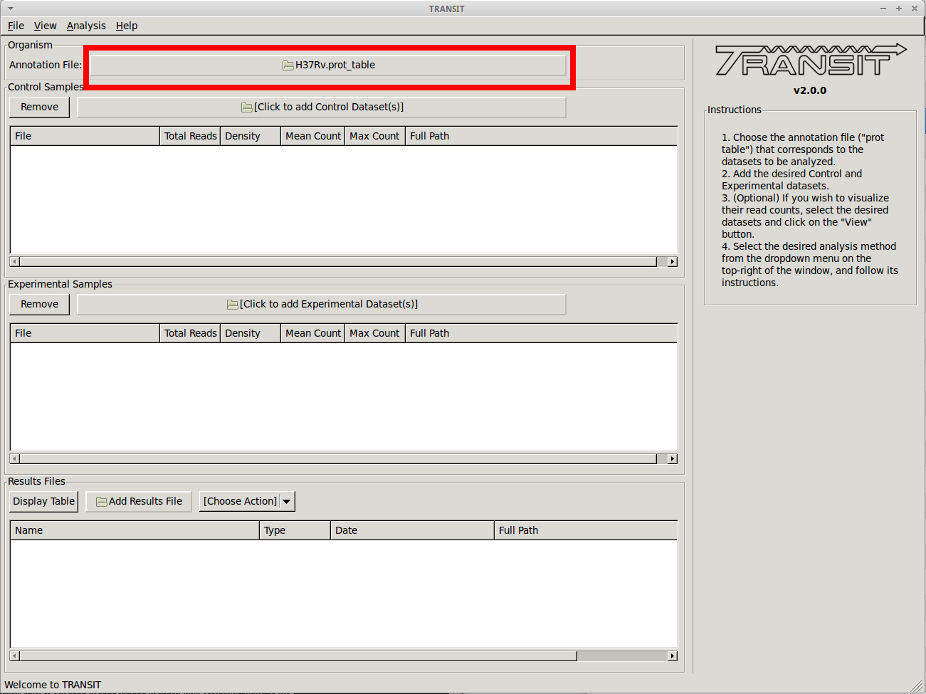
Adding the annotation file
Before we can analyze datasets, we need to add an annotation file for the organism corresponding to the desired datasets. Click on the file dialog button, on the top of the TRANSIT window (see image below), and browse and select the appropriate annotation file. Note: Annotation files must be in “.prot_table” format, described above.
Adding the control datasets
We want to analyze datasets grown in glycerol to those grown in cholesterol. We are choosing the datasets grown in glycerol as the “Control” datasets. To add these, we click on the control sample file dialog (see image below), and select the desired datasets (one by one). In this example, we have two replicates:
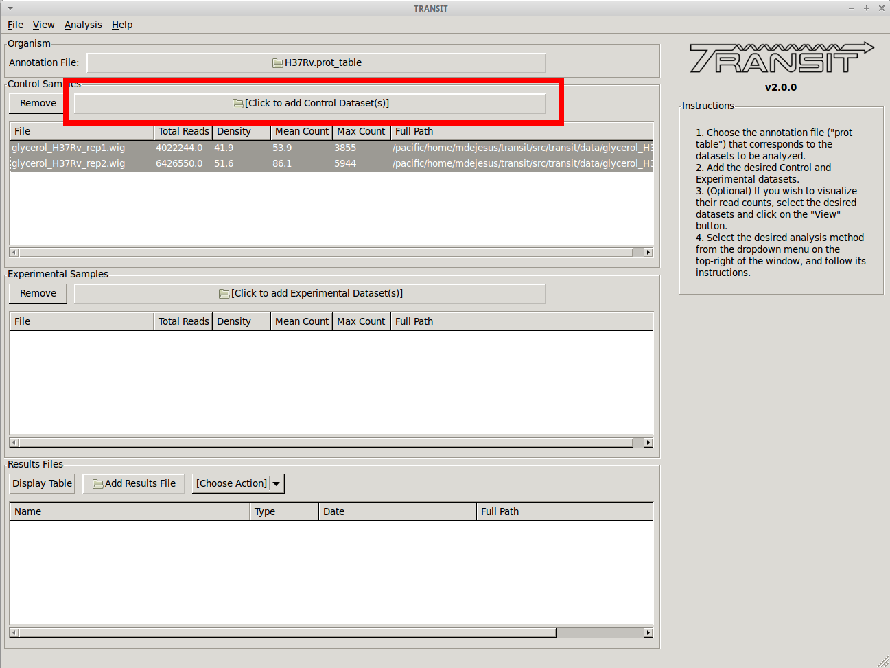
As we add the datasets they will appear in the table in the Control samples section. This table will provide the following statistics about the datasets that have been loaded so far: Total Number of Reads, Density, Mean Read Count and Maximum Count. These statistics can be used as general diagnostics of the datasets.
Visualizing read counts
TRANSIT allows us to visualize the read-counts of the datasets we have already loaded. To do this, we must select the desired datasets (“Control+Click”) and then click on “View -> Track View” in the menu bar at the top of the TRANSIT window. Only those selected datasets will be displayed:
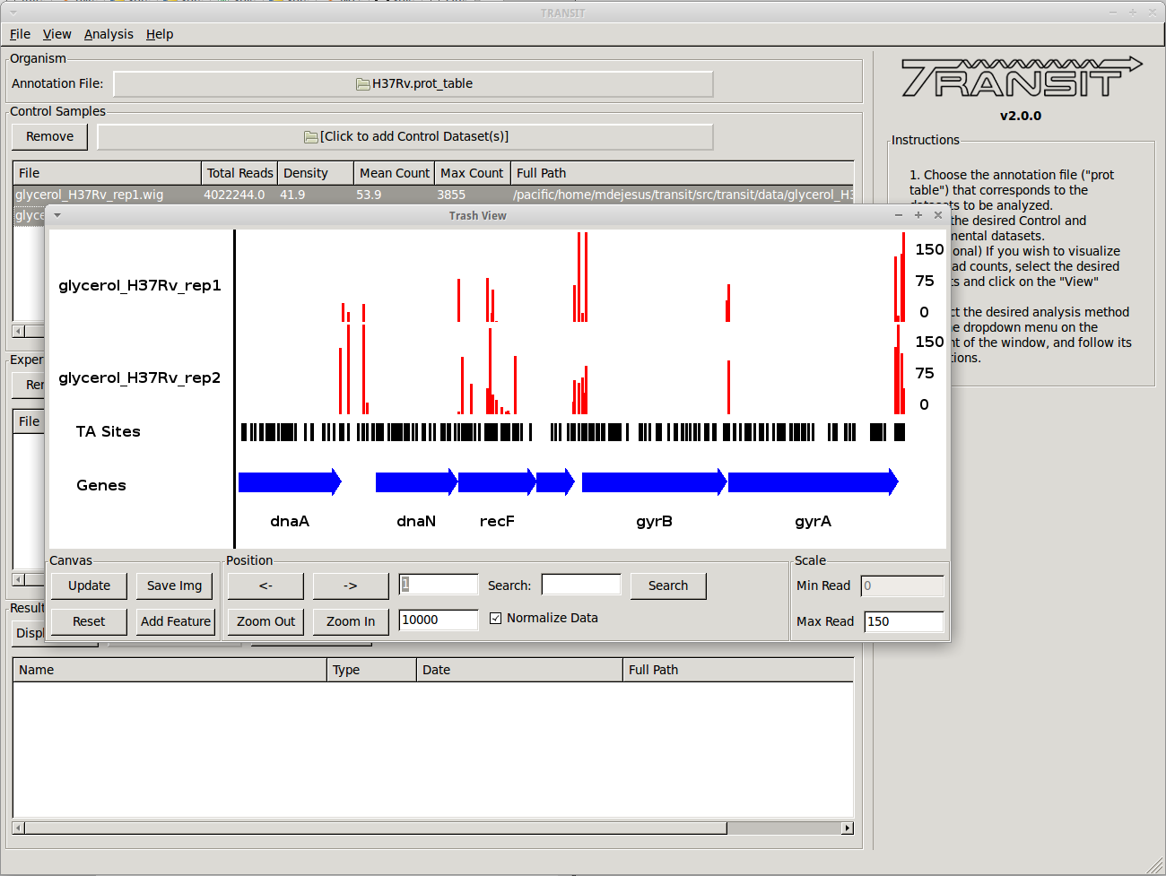
This will open a window that allows that shows a visual representation of the read counts at the TA sites throughout the genome. The scale of the read counts can be set by changing the value of the “Max Read” textbox on the right. We can browse around the genome by clicking on the left and right arrowm, or search for a specific gene with the search text box.
This window also allows us to save a .png image of the canvas for future reference if desired (i.e. Save Img button).
Scatter plot
We can also view a scatter plot of read counts of two selected datasets. To achieve this we select two datasets (using “Control + Clicck”) and then clicking on “View -> Scatter Plot” in the menu bar at the top of the TRANSIT window.
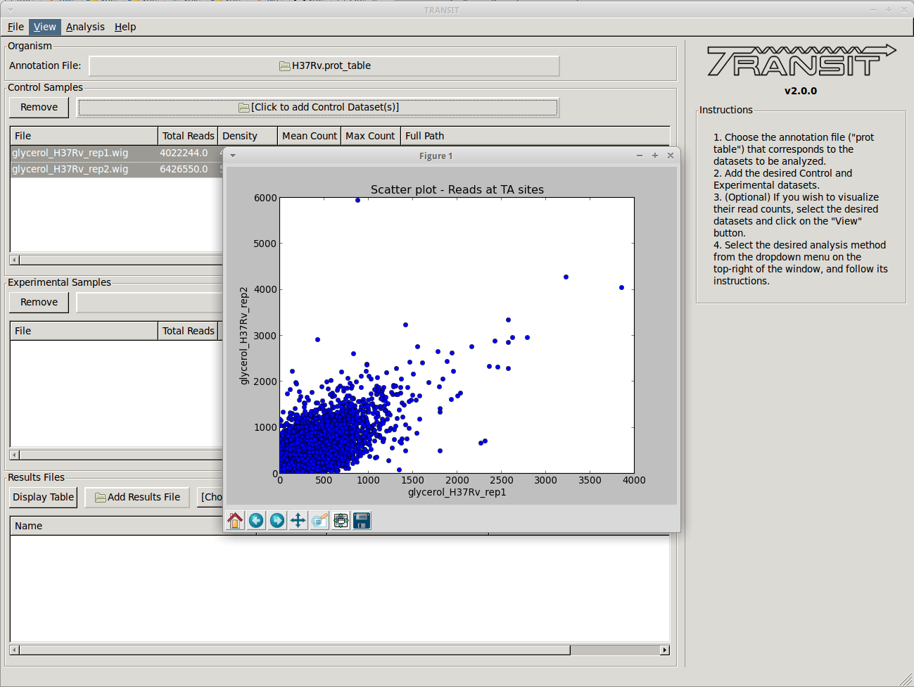
A new window will pop-up, show a scatter plot of both of the selected datasets. This window contains controls to zoom in and out (magnifying glass), allowing us to focus in on a specific area. This is particularly useful when large outliers may throw off the scale of the scatter plot.
Essentiality analysis with the Gumbel method
Before comparing both conditions against each other, we may want to determine which genes are essential in a specific condition to get an idea of the genes which are required. To do this we can use the Gumbel or the HMM methods, which determine essentiality within one condition. First we chose the Gumbel method from the list of (Himar1) analysis methods in the menu on top:
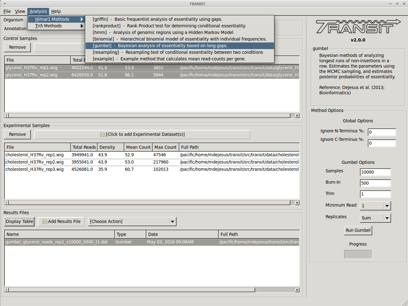
For this particular case we leave the parameters at their default settings as these work with a wide variety of datasets (See above for an explanation of their function). We then click on the “Run Gumbel” button and wait until the analysis finished running. The progress bar will give us information about how much of the analysis is still left. Once the program finishes, the results file is automatically created (with the name chosen at run-time) and it is automatically added to the Results File section at the bottom of TRANSIT. We can visualize the results by selecting this file from the list, and clicking on the “Display Table” button. This will open a new window with a table of resuls:
From this window we can view results, and sort on a specific column (described above) by clicking on a column header. In addition, the top of this window contains a breakdown of the number of essential and non-essential genes found by the Gumbel method. We can see that 675 genes are found to be essential by the Gumbel method (16%), roughly matching expectations that 15% of the genomes is necessary for growth in bacterial organisms. Clicking on the “Zbar” column we can sort the data on the posterior probability of essentiality. If we sort in descending order, we get those genes which are most likely to be essential on the top. Among these are genes like GyrA (DNA gyrase A) and RpoB (DNA-directed polymerase), which are both well-known essential genes, and which are obtain a posterior probability of essentiality of 1.0 (Essential).