CRISPRi-DR
CRISPRi-DR is designed to analyze CRISPRi libraries from CGI experiments and identify significant CGIs ie genes that affect sensitivity to the drug when depleted. [REF: TBA]
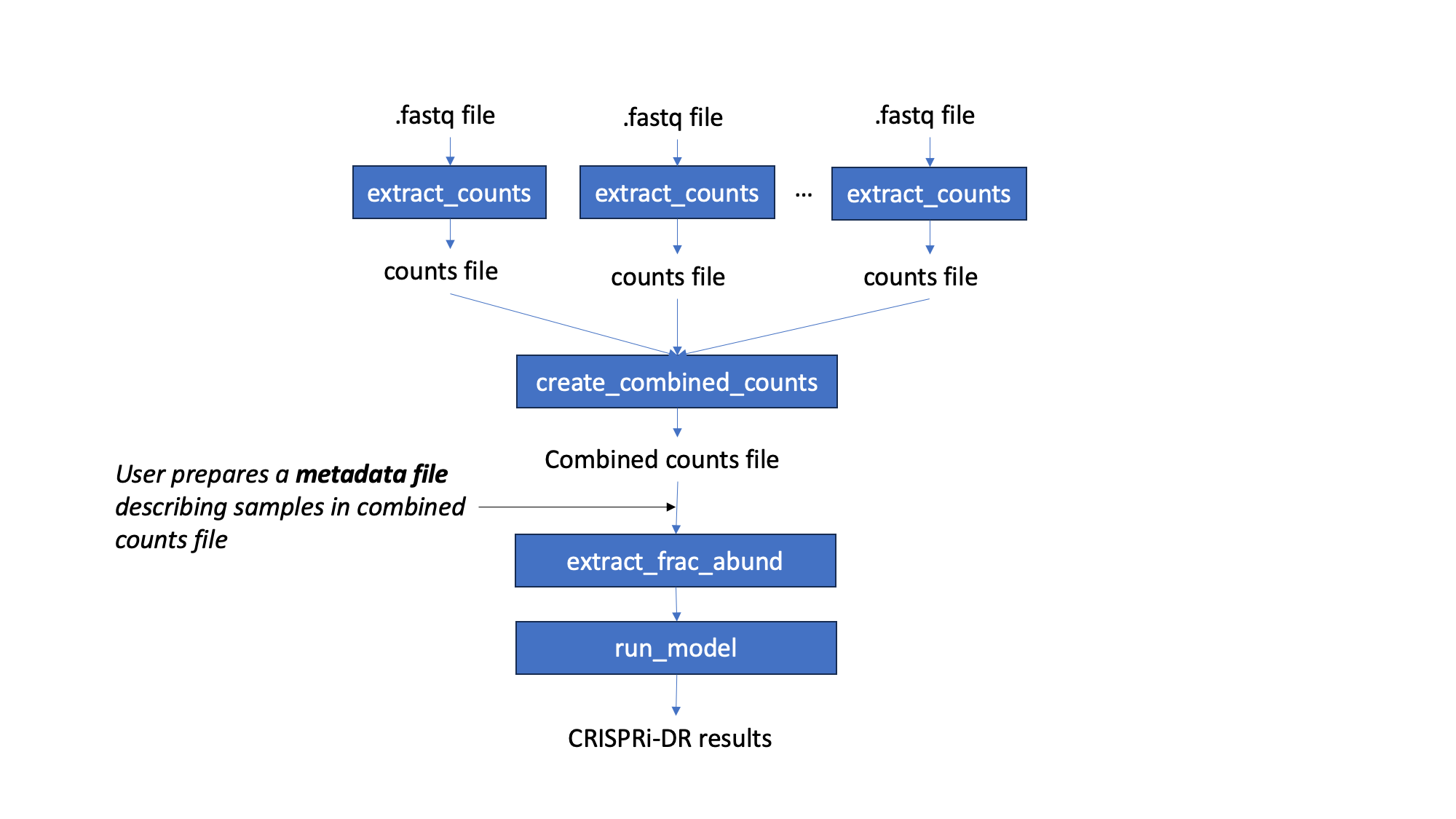
Workflow
Starting with fastq files, barcode counts are extracted. The user creates their own metadata file, for the counts. Fractional abundances are and used to run the CRISPRi-DR model. The output of this model is a file that lists genes with their statistacal parameters and significance. Genes with significant interactions are those with qval of condetration dependence < 0.05 and |Z score of concentration dpendence|>2 on the slope coefficient. However, genes can be ranked by depletion by sorting the coefficient of concentration dependence in ascending order
Preprocessing: Fastq to Count Files
This is a longer process, taking a few minutes each. However, the number of reads processed is printed to the console to indicate progress.
> python3 ../src/transit.py CGI extract_counts <fastq_file> <ids_file> > <counts_file>
- ids_fileList of sgRNAs used in the experiment, where each row is one sgRNA id.
For H37Rv experiments, the ids file is available in :
transit/src/pytransit/data/CGI/IDs.H37Rv.CRISPRi.lib.txt
Step 1: Combine Individual Counts File to a Combined Counts File This is a fairly fast process. It takes at most a minute for the combination of 12 files with 2 columns (sgRNA id and counts) to one large file of 13 columns (first column sgRNA id and remaining columns are counts from the files entered).
> python3 ../src/transit.py CGI combined_counts <comma seperated headers> <counts file 1> <counts file 2> ... <counts_file n> > <combined counts file>
counts files : sgRNA ids as their first column, and can have any number of columns.
- comma-separated headers: the column names of the combined counts file
Note
the comma-seperated headers must be in order of the columns in the count files(s) provided
Step 2: Extract Fractional Abundances
This is a relatively quick process, taking less than a minute. This step is to turn the barcodes counts into relative normalized abundances. Counts are normalized within samples and calculated relative to the abundances in the uninduced ATC file, essentially fractions. The first few lines of the output file contains information about the counts files processed.
> python3 ../src/transit.py CGI extract_abund <combined counts file> <counts metadata file> <control condition> <sgRNA strengths file> <uninduced ATC file> <drug> <days> > <fractional abundance file>
counts metadata file (USER created):
The columns expected in this file: column_name, drug, conc_xMIC, days_predepletion
column_name: the corresponding header name(s) in the combined counts file
conc_xMIC is the concentration of the drug the sample is treated with
Warning
conc_xMIC must be a numerical value, ie. 0.5 and not a categorical value such as “low” or “high”
Equal number of replicates for all concentrations are not nessessary
see [Li, S et al. 2022, PMID: 35637331] for explanation of days_predepletion
Example metadata:
transit/src/pytransit/data/CGI/counts_metadata.txt
control condition: The condition to to be considered the control for these set of experiments, as specificed in the “drug” column of the metadata file; typically an atc-induced (+ ATC) with 0 drug concentration condition.
sgRNA strengths file: A file that contains metadata for each sgRNA in the combined counts file, where the first column must be sgRNA id (as seen in the combined counts file) and the last column must be the strength measurement of the sgRNAs (in publication of this method, sgRNA strength is measurement as extrapolated LFCs calculated through a passaging experiment).
uninduced ATC file: A two column file of sgRNAs and their counts in uninduced ATC (no ATC) with 0 drug concentration
drug : Name of the drug in the “drug” column of the metadata file passed in to be fit in the model
days: Sampled from predepletion day as listed in the “days_predepletion” column of the metadata file to be used in the analysis
Step 3: Run the CRISPRi-DR model
This is a relatively quick process, taking at most 3 minutes for a dataset of ~90,000 sgRNAs . This step fits the CRISPRi-DR model (statistical analysis of concentration dependence for each gene) to each gene in the file and prints each output to the <CRISPRi-DR results file> in a tab seperated file.
> python3 ../src/transit.py CGI run_model <fractional abundance file> > <CRISPRi-DR results file>
Siginificant interacting genes are those with adjusted P-val (Q-val) < 0.05 and |Z slope| > 2, these are indicated by a “-1” for depleted and “1” for enriched in in the “Significant Interactions” column
Note
When the file is sorted on the slope of concentration dependence, the user can rank the genes based on amount of depletion.
Visualize Specific Genes
This process is fairly quick, taking less than a minute to run. This figure visualizes the amount of depletion in a gene at the sgRNA level. If control concentration provided is 0, the lowest value on the x-axis in the plot refers to this concentration (due to taking log concentration, 0 concentration is treated as a teo fold lower than the lowest concentration.) The slope of relative abundance (fraction of abundance of counts in ATC induced vs. ATC uninduced) versus log2(concentration) for each sgRNA is calculated and plotted, colored by sgRNA strenght based on a blue-orange gradient (as seen here):
> python3 ../src/transit.py CGI visualize <fractional abundance file> <gene> <output plot location>
fractional abundance file : Fractional abundance file as created in Step 2.
Warning
This visualization assumes the columns are in increasing order of concentration, with the first three abundance columns (after the column “sgRNA strength”), as the control. This order depends on the order of columns during the creation of the combined counts file in Step 1.
gene : select a gene to visualize. Use orf or gene name
output plot location : The location where to save the generated plot.
Note
If comparing plots from different genes, note the scale of sgRNA strength shown in the plots.
Tutorial
Data : Obtain FastQ files from NCBI using the following run numbers
Fetch and process the following fastq files from NCBI using the SRA toolkit and place them in the transit/src/pytransit/data/CGI directory :
FastQ files for the 3 replicates of control samples in this experiment. They are in a ATC-induced 0 drug concentration DMSO library with 1 day predepletion
SRR14827863 -> extracts SRR14827863_1.fastq
SRR14827862 -> extracts SRR14827862_1.fastq
SRR14827799 -> extracts SRR14827799_1.fastq
FastQ files for 3 replicates of high concentration RIF in a 1 day pre-depletion library
SRR14827727 -> extracts SRR14827727_1.fastq
SRR14827861 -> extracts SRR14827861_1.fastq
SRR14827850 -> extracts SRR14827850_1.fastq
FastQ files for 3 replicates of medium concentration RIF in a 1 day pre-depletion library
SRR14827760 -> extracts SRR14827760_1.fastq
SRR14827749 -> extracts SRR14827749_1.fastq
SRR14827738 -> extracts SRR14827738_1.fastq
FastQ files for 3 replicates of low concentration RIF in a 1 day pre-depletion library
SRR14827769 -> extracts SRR14827769_1.fastq
SRR14827614 -> extracts SRR14827614_1.fastq
SRR14827870 -> extracts SRR14827870_1.fastq
This tutorial shows commands relative to this directory. Other files in the transit/src/pytransit/data/CGI directory are:
counts_metadata.txt - describes the samples
sgRNA_metadata.txt - contains extrapolated LFCs for each sgRNA
uninduced_ATC_counts.txt - counts for uninduced ATC (no induction of target depletion) library
IDs.H37Rv.CRISPRi.lib.txt - ids of the sgRNAs that target the genes in H37Rv used in these experiments
Preprocessing: Fastq to Count Files
Create file of barcode counts from fastq files. Each fastq files reflect one replicate of a drug concentration, thus each will be converted into a file with two columns, sgNRA id and barcode counts
> python3 ../../../transit.py CGI extract_counts RIF_fastq_files/SRR14827863_1.fastq IDs.H37Rv.CRISPRi.lib.txt > DMSO_D1_rep1.counts
> python3 ../../../transit.py CGI extract_counts RIF_fastq_files/SRR14827862_1.fastq IDs.H37Rv.CRISPRi.lib.txt > DMSO_D1_rep2.counts
> python3 ../../../transit.py CGI extract_counts RIF_fastq_files/SRR14827799_1.fastq IDs.H37Rv.CRISPRi.lib.txt > DMSO_D1_rep3.counts

> python3 ../../../transit.py CGI extract_counts RIF_fastq_files/SRR14827769_1.fastq IDs.H37Rv.CRISPRi.lib.txt > RIF_D1_Low_rep1.counts
> python3 ../../../transit.py CGI extract_counts RIF_fastq_files/SRR14827614_1.fastq IDs.H37Rv.CRISPRi.lib.txt > RIF_D1_Low_rep2.counts
> python3 ../../../transit.py CGI extract_counts RIF_fastq_files/SRR14827870_1.fastq IDs.H37Rv.CRISPRi.lib.txt > RIF_D1_Low_rep3.counts

> python3 ../../../transit.py CGI extract_counts RIF_fastq_files/SRR14827760_1.fastq IDs.H37Rv.CRISPRi.lib.txt > RIF_D1_Med_rep1.counts
> python3 ../../../transit.py CGI extract_counts RIF_fastq_files/SRR14827749_1.fastq IDs.H37Rv.CRISPRi.lib.txt > RIF_D1_Med_rep2.counts
> python3 ../../../transit.py CGI extract_counts RIF_fastq_files/SRR14827738_1.fastq IDs.H37Rv.CRISPRi.lib.txt > RIF_D1_Med_rep3.counts

> python3 ../../../transit.py CGI extract_counts RIF_fastq_files/SRR14827727_1.fastq IDs.H37Rv.CRISPRi.lib.txt > RIF_D1_High_rep1.counts
> python3 ../../../transit.py CGI extract_counts RIF_fastq_files/SRR14827861_1.fastq IDs.H37Rv.CRISPRi.lib.txt > RIF_D1_High_rep2.counts
> python3 ../../../transit.py CGI extract_counts RIF_fastq_files/SRR14827850_1.fastq IDs.H37Rv.CRISPRi.lib.txt > RIF_D1_High_rep3.counts
Step 1: Combine Counts Files to a Combined Counts File
Combine the 12 seperate counts files into one combined counts file. Here we put the control samples first (DMSO) and then the drug-treated libraries (RIF) in increasing concentration
> python3 ../../../transit.py CGI create_combined_counts DMSO_D1_rep1,DMSO_D1_rep2,DMSO_D1_rep3,RIF_D1_Low_rep1,RIF_D1_Low_rep2,RIF_D1_Low_rep3,RIF_D1_Med_rep1,RIF_D1_Med_rep2,RIF_D1_Med_rep3,RIF_D1_High_rep1,RIF_D1_High_rep2,RIF_D1_High_rep3 DMSO_D1_rep1.counts DMSO_D1_rep2.counts DMSO_D1_rep3.counts RIF_D1_Low_rep1.counts RIF_D1_Low_rep2.counts RIF_D1_Low_rep3.counts RIF_D1_Med_rep1.counts RIF_D1_Med_rep2.counts RIF_D1_Med_rep3.counts RIF_D1_High_rep1.counts RIF_D1_High_rep2.counts RIF_D1_High_rep3.counts > RIF_D1_combined_counts.txt
The resulting file will have 13 columns, where the first column is sgRNA ids and the remaining are the counts for three replicates each for DMSO, RIF D1 Low Concentration, RIF D1 Med Concentration and RIF D1 High Concentration, respectively.
Step 2: Extract Fractional Abundances
Note
As a part of this step, the user must also generate a metadata file. , ie. counts_metadata.txt. Note the values in the conc_xMIC column is actual values (0.0625, 0.125, 0.25) and not categorical values (“low”, “medium”, “high”) as seen in the counts file names.
> python3 ../../../transit.py CGI extract_abund RIF_D1_combined_counts.txt counts_metadata.txt DMSO sgRNA_metadata.txt uninduced_ATC_counts.txt RIF 1 > RIF_D1_frac_abund.txt
The result of this command should be a file with a set of comments at the top, detailing the libraries used (DMSO and RIF). There should be a total of 17 columns, the last 12 of which are the calculated abundances, the first is the sgRNA ids followed by the orf/gene the sgRNA is targeting, uninduced ATC values, and sgRNA strength.
Step 3: Run the CRISPRi-DR model
> python3 ../../../transit.py CGI run_model RIF_D1_frac_abund.txt > RIF_D1_CRISPRi-DR_results.txt
There should be a total of 184 significant gene interactions, where 111 are significant depletions and 73 are significantly enriched.
Note
When the file is sorted on the slope of concentration dependence, the user can rank the genes based on amount of depletion.
Visualize Specific Genes
Here are a few samples of the interactions visualized at the sgRNA level for this experiment. Note the difference in sgRNA strength scales shown.
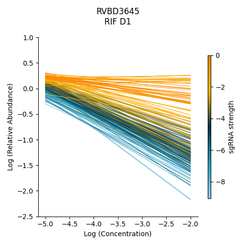
Significantly depleted gene : RVBD3645
RVBD3645 is one of the significantly depleted genes in this experiment. In this plot, notice how most of the slopes are negative but the amount of depletion varies, where the more blue slopes (higher sgRNA strength) are steeper than orange sgRNA slopes (lower sgRNA strength)
> python3 ../../../transit.py CGI visualize RIF_D1_frac_abund.txt RVBD3645 ./RVBD3645_lmplot.png
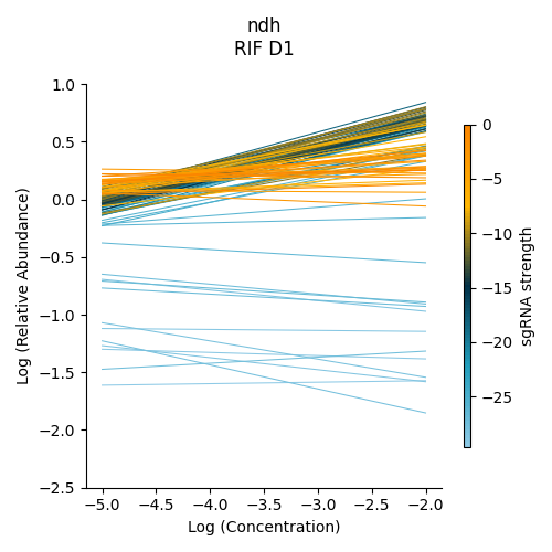
Significantly enriched gene : ndh
ndh is one of the signifincantly enriched genes in this experiment. In its plot, notice how sgRNAs of high strength (blue green ones) show a strong upwards trend but those will lower strength (the orange ones) do not. In fact there a few sgRNAs that show almost no change in fractional abundace as concentration increases.
> python3 ../../../transit.py CGI visualize RIF_D1_frac_abund.txt ndh ./ndh_lmplot.png #enriched
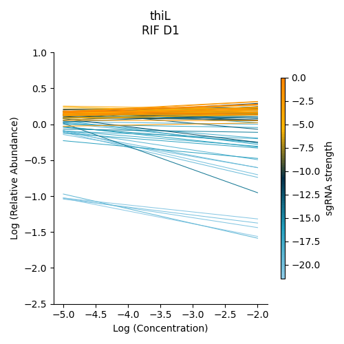
Non-interacting gene : thiL
thiL is an example on an non-interacting gene. It was found to be neither signifinicantly enriched nor depleted. Notice how in its plot, most of the slopes are fairly flat. As seen in the plots of RVBD3645 and ndh, the bluer slopes show greater depletion than the orange slopes, but there is no overall trend present
> python3 ../../../transit.py CGI visualize RIF_D1_frac_abund.txt thiL ./thiL_lmplot.png